Whether you like it or not, no one should ever claim to be a data analyst until he or she has done string manipulation.

I am reading Gaston Sanchez' book Handling and Processing Strings in R (pdf).

In the preface, I found the following quote, to which I wholeheartedly agree:

Perhaps even worse is the not so uncommon believe that string manipulation is a secondary non-relevant task. People will be impressed and will admire you for any kind of fancy model, sophisticated algorithms, and black-box methods that you get to apply. Everybody loves the haute cuisine of data analysis and the top notch analytics. But when it comes to processing and manipulating strings, many will think of it as washing the dishes or pealing and cutting potatos. If you want to be perceived as a data chef, you may be tempted to think that you shouldn’t waste your time in those boring tasks of manipulating strings. Yes, it is true that you won’t get a Michelin star for processing character data. But you would hardly become a good data cook if you don’t get your hands dirty with string manipulation. And to be honest, it’s not always that boring. Whether you like it or not, no one should ever claim to be a data analyst until he or she has done string manipulation.

Little things that make life easier #9: Using data.entry in r

With data.entry(), it's easy to visually fill (small) matrices in r.

Let's see it in action. First, I create a 4x3 matrix:

mx <- matrix(nrow=4, ncol=3) show(mx)

[,1] [,2] [,3] [1,] NA NA NA [2,] NA NA NA [3,] NA NA NA [4,] NA NA NA

The matrix is created with the cells' values being NA Now, in order to assign values to these cells, I use

data.entry(mx)

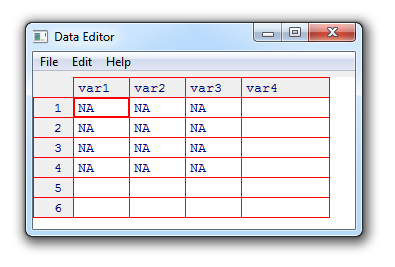
This opens a small window where I can enter the data.
This is how the cells were filled before my editing them:

And here's how they looked after my editing them just before I used File > Close:

Back in the shell, the matrix has indeed changed its values:

show(mx)

var1 var2 var3 [1,] 2 4 2 [2,] 12345 8 42 [3,] 5 6 489 [4,] 9 22 11

Pretty cool, imho.

The power of k-nearest-neighbor searches

I came across the k-nearest-neighbor (k-NN) algorithm recently. Altough it's a relatively simple algorithm, its power still amazed me.

K-NN can be used to classify sets of data when the algorithm is fed with some examples of classifications.

In order to demonstrate that, I have written a perl script. The script creates two csv files (known.csv and unknown) and a third file: correct.txt. The k-NN algorithm will use known.csv to train its understanding of a classification. Then, it tries to guess a classification for each record in unknown.csv. For comparing purposes, correct.txt contains the classification for each record in unknown.csv.

Structure of known.csv

known.csv is a csv file in which each record consists of 11 numbers. The first number is the classifaction for the record. It is a integer between 1 and 4 inclusively. The remaining 10 numbers are floats between 0 and 1.

Structure of unknown.csv

In unknown.csv, each record consists of 10 floats between 0 and 1. They correspond to the remaining 10 numbers in known.csv. The classification for the records in unkown.csv is missing in the file - it is the task of the k-NN algorithm to determine this classification. However, for each record in unknown.csv, the correct classification is found in correct.txt

Values for the floats

A record's classification determines the value-ranges for the floats in the record, according to the following graphic:
The four classifications are represented by the four colors red, green, blue and orange. The Perl script generated eight floats. For range for the first float for the red classification is [0.15,0.45], the range for the first float for the green classification is [0.35,0.65] etc. Similarly, the range for the second value of the red classification is [0.55,0.85] and so on.

To make things a bit more complicated, two random values in the range [0,1] are added to the eight values resulting in 10 values. These two values can either be at the beginning, at the end or one at the beginning and the other at the end.

Result

When I let the Perl script create 1000 unknown and known records, the following r script guesses more than 985 classifications right, most of the time.

library(FNN) known <- read.csv("known.csv" , header=FALSE) unknown <- read.csv("unknown.csv", header=FALSE) labels <- known[, 1] known <- known[,-1] results <- (0:4)[knn(known, unknown, labels, k = 10, algorithm="cover_tree")] write(results, file="guessed.txt", ncolumns=1)

Links

Source code on github

I find that rather impressive