OpenStreetMap: convert an pbf to an sqlite database with Python

Recently, I have demonstrated how the open street map pbf parser (OSMpbfParser.py) can be used to create xml files. With little effort, a script can be written that creates and fills an sqlite database. Of course, I first have to define a schema into which I load the data. I think this is also a good exercise to understand the internals of osm data. The tables are adapted from the original open street data database schema.

Tables

Table node

The node table is the fundamental table for open street map. Each node consists of a longitude (lon) / latitude (lat) pair and thus defines a geographical point on the surface of the earth. The original schema has a few more attributes, such as changeset_id or version. I am not interested in these, so I don't load them:

create table node( id integer primary key, lat real not null, lon real not null );

Tables way and node_in_way

Each "line" (such as a street or border etc) on open street map is an ordered list of nodes. Open Street Map calles them ways. Ways are also used to define areas in which case the last node equals the first node in the list.

First, I need a table just to store each way. Again, I am not interested in attributes such as user or changeset, so I just load the way's id:

create table way( id integer primary key );

The table node_in_way relates nodes and ways:

create table node_in_way( way_id integer not null references way deferrable initially deferred, node_id integer not null references node deferrable initially deferred, order_ integer not null )

Tables relation and member_in_relation

Open Street Map allows to relate multipe nodes and ways (and even relations) in a relation:

create table relation( id integer primary key );

Each member (that is either node, way or relation) is listed in member_in_relation. Thus, exactly one of the attributes node_id, way_id or relation_id is not null:

create table member_in_relation( id_of_relation integer not null references relation deferrable initially deferred, node_id integer null references node deferrable initially deferred, way_id integer null references way deferrable initially deferred, relation_id integer null references relation deferrable initially deferred, role text )

Table tag

Finally, there are tags. A tag is a key (k) value (v) pair that can be assigned to nodes, ways or relations. Often, the values for specific keys define what an object is. As in member_in_relation exactly on of node_id, way_id or relation_id is not null.

create table tag( node_id integer null references node deferrable initially deferred, way_id integer null references way deferrable initially deferred, relation_id integer null references relation deferrable initially deferred, k text not null, v text not null )

ERD

Here's the ERD for these tables:

The ERD was created with dia from pbf2sqlite-erd.dia.

Loading the pbf to a sqlite db

In order to run the script, a pbf must be obtained, for example with download-switzerland-pbf.py.

Then, this pbf can be loaded into a sqlite db on the command line with

pbf2sqlite.py xyz.pbf xyz.db

The script is on github: pbf2sqlite.py.

Links

Parsing an Open Street Map pbf file with Python

Open Street Map: convert pbf to xml

A Google Earth hiking map for the Säntis region with Open Street Map data

An open street map node density map for Switzerland

Why is there no == operator in SQL?

Why is there no == operator in SQL that yields true if both operands are either null or have the same value?

Here's the truth table for the = operator:

=	42	13	null
42	true	false	null
13	false	true	null
null	null	null	null

This has some implications. The statement

select * from t where col1 = col2

won't return a record where both col1 and col2 are null.

I suspect that in most cases this is not what the author of such a statement wants. Therefore, they will rewrite the query so:

select * from t where ( a is null and b is null) or ( a = b)

Now, if there were a == operator with this truth table:

==	42	13	null
42	true	false	false
13	false	true	false
null	false	false	true

it would definitely make my life easier (and would not cost the database companies too much money to implement).

Maybe I am all wrong and there is such a thing somewhere. If you know of such an operater in any database product, please let me know!

Oh that pesky Oracle outer join symbol (+)

Here are three tables, named A, A2Z and Z that I want to outer join from left to right:

The first table, A, contains the (primary keys) 1 through 7. I want my select to return each of these, that's why I use an outer join. A's column i is outer joined to A2Z's column ia:
A.i = A2Z.ia (+).
The (+) symbol indicates that a record should be returned even if there is no matching record. Note, the (+) is on the side of the = where "missing" records are expected.

Now, the records in A2Z should be joined to Z if A2Z's column flg is equal to y (colored green in the graphic above). For example, for the 1 in A, I expected the query to return the a in Z, for the 2 in A I expect no matching record in Z since the corresponding flg is either null or not equal to y.
This requirement can be implemented with a
A2Z.flg (+) = 'y'
Note, the (+) is on the side where missing records (or null values) are expected. Since y is neither missing nor null, it goes to the other side.

Finally, A2Z needs to be joined to Z:
A2Z.iz = Z.i (+)

Complete SQL Script

create table A (i number(1) primary key); create table Z (i char (1) primary key); create table A2Z ( ia not null references A, flg char(1) not null, iz char(1) not null ); insert into A values (1); insert into A values (2); insert into A values (3); insert into A values (4); insert into A values (5); insert into A values (6); insert into A values (7); insert into Z values ('a'); insert into Z values ('b'); insert into Z values ('c'); insert into Z values ('d'); insert into A2Z values (1, 'y', 'a' ); insert into A2Z values (1, 'n', 'b' ); insert into A2Z values (2,null, 'c' ); insert into A2Z values (2, 'q', 'd' ); insert into A2Z values (3, 'y', 'e' ); insert into A2Z values (4, , 'f' ); insert into A2Z values (5, 'y', null); insert into A2Z values (6, 'v', null); select A.i a_i, Z.i z_i from A, A2Z, Z where A.i = A2Z.ia (+) and A2Z.flg (+) = 'y' and A2Z.iz = Z.i (+) order by A.i; drop table A2Z purge; drop table Z purge; drop table A purge;

When run, the select returns the following records:

       A_I Z
---------- -
         1 a
         2
         3
         4
         5
         6
         7

Links

Source code on github

Little things that make live easier #1: convert an svg file to a png on the command line with inkscape

Inkscape can be used to create pngs (or other image formats) on the command line:

c:\foo\bar> inkscape -f input.svg -e output.png

Of course, this works with inkscape files, too...

Open Street Map: convert pbf to xml

Here's an example on how the open street map parser can be used to create xml files. Please excuse the wide source...

import sys import time import OSMpbfParser def xml_escape(s_): s_=s_.replace ("&", "&" ) s_=s_.replace ("<", "<" ) s_=s_.replace (">", ">" ) s_=s_.replace ('"', '"') return s_ def callback_node(node): stamp=time.strftime("%Y-%m-%dT%H:%M:%SZ",time.gmtime(node.time)) if len(node.Tags)>0: fh.write(' \n' % (node.NodeID, node.version, stamp, node.uid, xml_escape(node.user), node.changeset, node.Lat, node.Lon)) for t in node.Tags.keys(): fh.write(' \n' % (t, xml_escape(node.Tags[t]))) fh.write(' \n') else: fh.write(' \n' % (node.NodeID, node.version, stamp, node.uid, xml_escape(node.user), node.changeset, node.Lat, node.Lon)) def callback_way(way): stamp=time.strftime("%Y-%m-%dT%H:%M:%SZ",time.gmtime(way.time)) fh.write(' \n' % (way.WayID, way.version, stamp, way.uid, xml_escape(way.user), way.changeset)) for n in way.Nds: fh.write(' \n' % (n)) for t in way.Tags.keys(): fh.write(' \n' % (t,xml_escape(way.Tags[t]))) fh.write(' \n') def callback_relation(relation): stamp=time.strftime("%Y-%m-%dT%H:%M:%SZ",time.gmtime(relation.time)) fh.write(' \n' % (relation.RelID, relation.version, stamp, relation.uid, xml_escape(relation.user), relation.changeset)) for m in relation.Members: fh.write(' \n' % (m.type, m.ref, xml_escape(m.role))) for t in relation.Tags.keys(): fh.write(' \n' % (t,xml_escape(relation.Tags[t]))) fh.write(' \n') # First argument is *.pbf file name pbf_filename = sys.argv[1] # Second (optional) argument is output file if len(sys.argv) > 2: fh = open(sys.argv[2], 'w') else: fh = sys.stdout fh.write('\n') fh.write('\n') OSMpbfParser.go(pbf_filename, callback_node, callback_way, callback_relation) fh.write('\n') fh.close()

This script takes one mandatory and an optional argument. The mandatory argument specifies the pbf file. If the optional parameter is given, it specifies the name of the xml file into which the output is written, otherwise, the output goes to stdout:

c:\> pbf2xml.py liechtenstein-latest.osm.pbf liechtenstein.xml

Links

Source code on github

open street map parser

OpenStreetMap: convert an pbf to an sqlite database with Python

Parsing an Open Street Map pbf file with Python

Chris Hill at http://pbf.raggedred.net/ has written a parser in Python for open street map pbf files. His parser is free software, so I used this liberty to adapt it for my needs. In particular, his script either collects osm node, way and relation data either in memory (which is a problem for big pbf files) or it emits xml files with the osm data. I have changed his script so that I can pass three callback functions that are invoked as soon as the parser finished with one of the three fundamental osm type node, way or relation.

Here's a template that can be used to write a script that uses my adaption of the parser:

import OSMpbfParser def callback_node(node): do_something_with(node) def callback_way(way): do_something_with(way) def callback_relation(relation): do_something_with(relation) OSMpbfParser.go( 'the-file-to-be-parsed.pbf', callback_node, callback_way, callback_relation)

Each of the callback functions has exactly one parameter that corresponds to the classes OSMNode, OSMWay and OSMRelation (see the source at github).

Installing google's protocol buffers

To parse pbf files, google's protocol buffers are needed. The can be optained from code.google.com/p/protobuf/downloads/list.
For Windows, I downloaded protoc-2.5.0-win32.zip which contains one file: protoc.exe. After extracting this file, the environment variable PATH should be changed so that it points to the directory with protoc.exe.

For the python installation, the full source protobuf-2.5.0.tar.bz2 is also needed. After extracting them, cd into the python directory and execute:

cd protobuf-2.5.0\protobuf-2.5.0\python python setup.py build python setup.py test python setup.py install

Links

Source code on github

convert pbf files to xml

OpenStreetMap: convert an pbf to an sqlite database with Python

Creating a simple TopoJSON map

I want to create a simple map for a country (perhaps an island) that consists of three regions. Here's how this country looks like:
The three regions are confined by what TopoJSON refers to as arcs: A red arc to the West, an orange arc to the North East, a blue arc to the South east, and a light blue, a purple and a green arc going to the center of the country. To draw the map with these regions, I need to create a TopoJSON topology object. Usually, this object is specified in JSON, but for simplicity's sake, I just create an ordinary JavaScript object. This JavaScript object has a member arcs that is an array.

arcs: [ ..... ]

For each arc in the map, another array is inserted into this arcs: array:

arcs: [ [ ... ], // Red arc [ ... ], // light blue arc [ ... ], // orange arc /* etc */ ]

The elements in these nested arrays deteremine the coordinates of the respective arc. These coordinates are specified in a special format: the first element is the absolute coordinates and the following coordinates are relative to their previous coordinates. I hope the following picture makes this a bit clearer:

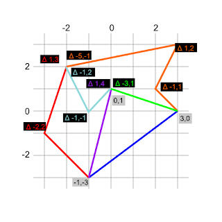
The red arc starts at -1,-3 and goes to -3,-1 which is -2,2 relative to the first coordinate. The third (and last) coordinate is relative 1,3 to the second coordinate. Hence, the entries in the arcs array become:

arcs: [ [ // Red arc [-1, -3], [-2, 2], [ 1, 3] ], [ // light blue arc [ .. ], [ .. ] ] /* etc */ ]

We can now refer to one of these arcs with an integer. The first arc is 0, the second 1 etc. If we want to refer to one of these arcs against its direction, the integer for the first arc is -1, for the second arc, its -2 etc. This allows us to define the regions with the integers for the respective confining arc. For example, the first region looks like

{ id: 'foo', type: 'Polygon', arcs: [ [0, -2, -5] ] },

This indicates that the region with id=foo is confined by the first arc (0) in direction of the arc, the second arc (-2, note the negative sign) against the direction of the arc (negative sign!) and the fifth arc (again against its direction, negative sign). Finally, the country (or island) needs to be placed somewhere on the earth. The latitute-spread of the Northernmost and Southernmost point of the country is 20 degrees, therefore, the scale is

scale: [ 10/3, 10/3 ]

The middle of the country is 45 degrees north and 0 degrees west, so the translation becomes

translate: [0, 45]

So, the complete TopoJSON object for the country looks like this:

topology = { type: 'Topology', objects: { regions: { type: 'GeometryCollection', geometries: [ {id: 'foo', type: 'Polygon', arcs: [ [0, -2, -5] ] }, {id: 'bar', type: 'Polygon', arcs: [ [3, 1, -3 ] ] }, {id: 'baz', type: 'Polygon', arcs: [ [ -6, 4, -4 ] ] } ] } }, arcs: [ [ // Red arc # 0 / -1 { [-1, -3], [-2, 2], [ 1, 3] ], // } [ // light blue arc # 1 / -2 { [ 0, 1], [-1, -1], [-1, 2] ], // } [ // orange arc # 2 / -3 { [ 3, 0], [-1, 1], [ 1, 2], [-5,-1] ], // } [ // green arc # 3 / -4 { [ 3, 0], [-3, 1] ], // } [ // purple arc # 4 / -5 { [ -1, -3], [ 1, 4] ], // } [ // blue arc # 5 / -6 { [ -1, -3], [ 4, 3] ] // } ], transform: { scale: [ 10/3, 10/3 ], translate: [0, 45] } }

To show this topology with d3.js, the folllowing code should do:

var width = 1000; var height = 500; var projection = d3.geo.albers() .center([0, 45]) .rotate([0,0]) .parallels([ 5,9]) .scale(1000) .translate([width / 2, height / 2]); // Create «SVG window» var svg = d3.select("body").append("svg").attr("width", width ).attr("height", height); // Create path generator var path = d3.geo.path().projection(projection).pointRadius(2); var regions = topojson.feature(topology, topology.objects.regions); svg.selectAll(".region") .data(regions.features) .enter().append("path") .attr("class", function(d) { return "region-" + d.id; }) .attr("d" , path);

Some CSS to change the colors of the regions:

svg { background-color: #eee; } path { stroke: #444; stroke-width:2px; } .region-foo { fill: #7ad; } .region-bar { fill: #d77; } .region-baz { fill: #da7; }

The complete html file is on github, as well as the inkscape/svg file for the graphics.

A simple bar chart with d3.js

With d3.js it is surprisingly simple to create a bar chart:

d3.select('.bar-chart').
  selectAll('div').
  data([194, 52, 228, 268, 163, 138, 92]).
  enter().
    append('div').
    style ('width', function(d) {return d + "px"}).
    text  (         function(d) {return d       });

For each of the data-elements (194, 52, 268 etc), a new div is appended with its css width style set to the respective px width. Since the divs are transparent per default, a bit of css is needed to make them visible:

.bar-chart div {
  background-color:#fa5;
  margin: 2px;
  color: #713;
  text-align: right}

Result:

github link

python -m SimpleHTTPServer

I wish I had known this earlier. With python installed, a simple webserver can be started on the command line with just a
python -m SimpleHTTPServer

This command creates a webserver that listens on port 8000, so that it can be accessed with a browser on localhost:8000
The command also accepts an alternative port instead the default 8000:

python -m SimpleHTTPServer 7777

github link

Sihleggstrasse 23, 8832 Wollerau

Switzerlands Zefix, the central index of companies (zentraler Firmenindex), is downloadable with FTP. This is of course an invitation to create a script that determines the address at which most Swiss companies are registered. Not surprisingly, this is in Wollerau, more precisly at

Sihleggstrasse 23
8832 Wollerau

At this address, 328 companies are registered!
For the reference, here's the list of the top twenty company addresses in Switzerland:

Registered companies	Street	Location
328	Sihleggstrasse 23	8832 Wollerau
304	Murbacherstrasse 37	6003 Luzern
222	Technoparkstrasse 1	8005 Zürich
203	Gewerbestrasse 5	6330 Cham
201	Baarerstrasse 75	6300 Zug
201	Chamerstrasse 172	6300 Zug
188	Neuhofstrasse 5A	6340 Baar
185	Industriestrasse 47	6300 Zug
182	Chemin du Château 26 A	2805 Soyhières
163	Riva Albertolli 1	6900 Lugano
162	Haldenstrasse 5	6340 Baar
157	Churerstrasse 35	9470 Buchs
157	Dammstrasse 19	6300 Zug
156	Rue du Rhône 100	1204 Genève
156	Weissbadstrasse 14	9050 Appenzell
149	Poststrasse 6	6300 Zug
148	Baarerstrasse 78	6300 Zug
145	Industriestrasse 21	6055 Alpnach Dorf
144	Oberneuhofstrasse 5	6340 Baar
140	Baarerstrasse 2	6300 Zug

Note how many companies are registered in Zug.

Sorting à la sqlite

Here's a sqllite table

create table dattyp (
  without_dt,
  dt_int integer,
  dt_text text)

The first column (without_dt) does not have an associated datatype with it, the second and third columns do: integer and text, respectively.
Let's fill the table with some values:

insert into dattyp values ( 2,  2,  2)
insert into dattyp values ( 9,  9,  9)
insert into dattyp values (19, 19, 19)

Check the sorting behavior: is it dependent on the datatype?

select without_dt from dattyp order by without_dt

2
9
19

select dt_int from dattyp order by dt_int

2
9
19

select dt_text from dattyp order by dt_text

19
2
9

Columns without explicit datatypes and integer columns are sorted numerically, while the text column is sorted alphanumerically.
Strings that can be converted to integers are inserted:

insert into dattyp values ('28', '28', '28')

Same sort check as above:

select without_dt from dattyp order by without_dt

2
9
19
28

select dt_int from dattyp order by dt_int

2
9
19
28

select dt_text from dattyp order by dt_text

19
2
28
9

The sorting behavior didn't change. Inserting strings that cannot be converted to an integer. Note that the strings can be inserted to the integer column as well:

insert into dattyp values ('foo', 'bar', 'baz')

Again the same selects:

select without_dt from dattyp order by without_dt

2
9
19
28
foo

select dt_int from dattyp order by dt_int

2
9
19
28
bar

select dt_text from dattyp order by dt_text

19
2
28
9
baz

A complete python script is in this github file

Codesnippet for using sqlite with Python

This is a code snippet intented to demonstrate the use use of the sqlite3 module in Python:

import sqlite3
import os.path

if os.path.isfile('foo.db'):
   os.remove('foo.db')

db = sqlite3.connect('foo.db')

cur = db.cursor()

cur.execute('create table bar (a number, b varchar)')

cur.execute("insert into bar values (2, 'two')")

cur.execute('insert into bar values (?, ?)', (42, 'forty-two'))

cur.executemany('insert into bar values (?, ?)', [
  (4, 'four'),
  (5, 'five'),
  (7, 'seven'),
  (9, 'nine')
])

for row in cur.execute('select * from bar order by a'):  
    print "%2d: %s" % (row[0], row[1])

Github link to script

Python: reading a csv file

Here's a csv file:

col 1,col 2,col 3
foo,bar,baz
one,two,three
42,,0 

This file can be read in python with this script:

import csv

csv_file   = open('data.csv', 'r')
csv_reader = csv.reader(csv_file)

header = csv_reader.next()

for record in csv_reader:
    
    print 'Record:'
    
    i = 0
    for rec_value in record:
        print '  ' + header[i] + ': ' + rec_value
        i += 1 

Github links: data.csv and script.py.

Python: How to download a gz file and decompress it in one go

Here's a python snippet I recently used that downloads .gz files from a ftp server and decompresses it in one go.

import zlib from ftplib import FTP def get_gz(ftp, ftp_filename, local_filename): decomp = zlib.decompressobj(16+zlib.MAX_WBITS) unzip = open (local_filename, 'wb') def next_packet(data): unzip.write(decomp.decompress(data)) ftp.retrbinary('RETR ' + ftp_filename, next_packet) decompressed = decomp.flush() unzip.write(decompressed) unzip.close() ftp_ = FTP('ftp.host.xyz') ftp_.login() ftp_.cwd('/foo/bar') get_gz(ftp_, 'remote-file.gz', 'local-file')

Link to github gist